In the complex interplay between supply and demand, customer requirements and a company’s ability to meet them are crucial factors. Here, capacity and demand analysis becomes a pivotal function. This systematic method ensures operational efficiency by accurately aligning the company’s production capabilities with customer demand.

Understanding the Dynamics of Capacity and Demand

At the heart of business process management, capacity symbolizes the zenith of output our systems, workforce, and resources can achieve within a set timescale. It’s a measure of potential, determining how much can be accomplished when our facilities operate with full force. In contrast, demand embodies the volume of work or resources our clientele mandates, regardless of our maximum production limit.

Navigating Bottlenecks: The Role of Analysis

The term ‘bottleneck’ is not merely industrial jargon but a frequent challenge in the domain of process management, where tasks queue up, awaiting their turn in the production pipeline. To prevent such congestion, capacity and demand analysis steps in as the arbiter of flow, ensuring the current is not a small or large quantity, but instead perfectly proportioned for optimal efficiency.

Taking Action: Steps for Effective Analysis

To embark on this analytical journey, one must:

• Identify the processes and resources ripe for review.
• Assess the current capacity of these elements.
• Estimate both present and future demand using billing trends and market exploration.
• Contrast and harmonize capacity with demand to pinpoint discrepancies and opportunities for enhancement.

This systematic method is not just about meeting the present needs but also about envisioning the future landscape of market demand and preparing to confront directly.

Calculating Capacity: The Interplay of BPMN, Resources, and Time

Determining capacity in Business Process Management (BPM) is like planning for a successful performance where each participant plays a crucial role in achieving the desired outcome. Here are the steps to follow for a capacity calculation based on BPM principles.

BPMN As-Is Model Assessment:

Begin with a thorough evaluation of the current state, or ‘As-Is’ model, of your business processes using Business Process Model and Notation (BPMN). This visual representation lays out the existing workflow, including all tasks, sequence flows, events, and gateways. This model sets the foundation for identifying the capacity by highlighting the resources currently in play.

Team and Machinery Evaluation:

With the ‘As-Is’ model as your guide, dissect the process to list down all human and machinery resources involved. Evaluate the efficiency of your team, their working hours, and the machinery’s operational capacity. The goal here is to quantify the productive output possible by both human and mechanical actors within a given time frame.

Time Management Considerations:

Cycle Time: Measure the time taken for a single process cycle from start to finish. This includes the active working time on a task without interruptions.

Waiting Time: Account for the duration a task spends idle, awaiting the next step in the process. This could be due to upstream delays or scheduling gaps.

Lead Time: The overall time from the initiation of the process to its completion, including both cycle and waiting times.

Process Bottlenecks and Capacity:

The BPMN model will often reveal points of congestion; bottlenecks where capacity is limited. It’s essential to assess how these chokepoints affect overall capacity. For instance, if a critical machine only operates at half the time it’s available due to maintenance issues, the capacity calculation must reflect this reduced availability.

Quantifying Capacity:

To quantify capacity, consider the formula:

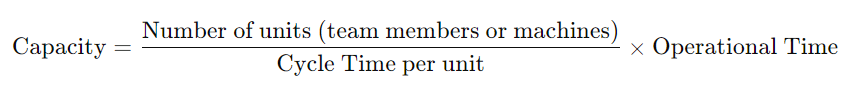
This calculation must be repeated for each critical resource, and the process’s overall capacity will be constrained by the resource with the lowest capacity, typically found at the bottleneck.

Adjusting for Real-World Scenarios:

Remember, theoretical capacity is not always realizable in practice. Factor in breaks, maintenance, unexpected delays, and other real-world scenarios that might affect capacity.

By understanding and applying these principles, you align capacity calculations with the BPMN As-Is model’s practical insights, account for the human and machine contributions, and acknowledge the time nuances. This comprehensive view not only quantifies your current capacity but also sets the stage for addressing and mitigating process bottlenecks.

Example of capacity calculation

To illustrate a capacity calculation for a clinical laboratory’s primary process of blood sample analysis, let’s walk through an example:

Daily Reception Capacity:

• Number of Receptionists: 3
• Time per Patient for Reception: 5 minutes

Each receptionist can see 12 patients per hour, which results in:

For all receptionists together:

Daily Blood Collection Capacity:

• Number of Technicians for Collection: 3
• Time per Patient for Collection: 7 minutes

Each technician can process about 8.57 patients per hour, resulting in:

For all technicians together:

Analysis Capacity Over Three Days:

• Number of Lab Technicians: 1
• Number of Equipment: 4 (operated simultaneously)

Time per Analysis: 2 hours

In one day, considering two-hour analyses, each piece of equipment can perform four analyses (since 2 hours x 4 = 8 hours), so all four can perform:

Over three days, this would be:

Summary of Daily Capacities:

• Reception can handle up to 288 patients per day.
• Blood collection can process up to 204 patients per day.

Analysis is capable of handling 16 analyses per day, totaling 48 analyses over a three-day period.

Even though the reception and collection processes have the capacity to handle a high volume of patients daily, the bottleneck in this scenario is the analysis stage.

The laboratory’s overall throughput is capped at 16 complete blood sample analyses per day, amounting to 48 analyses over a three-day period. This capacity is defined by the number of available equipment pieces and their operational time limits.

Mastering Market Demand: Calculating Today and Forecasting Tomorrow
In any service or production environment, demand calculation and estimation serve as critical functions to align operational capacity with market needs. These methodologies enable organizations to gear up for future requirements, ensuring that resources are aptly allocated, and customer satisfaction is maintained. Let’s delve into the conceptual approach of these two vital processes.

Demand Calculation: The preparation for growth

The calculation of demand is an empirical process, reliant on quantitative data from past and present interactions with the market. It involves the meticulous compilation and analysis of historical sales figures, service usage rates, customer orders, and transaction volumes. This retrospective examination sheds light on existing consumption patterns, providing a tangible metric that reflects the actual demand experienced by an organization.

Unlocking the Power of Data: Advanced Statistical Techniques for Demand

Forecasting

When it comes to leveraging historical data for demand calculation and forecasting, statistical methods play an fundamental role in extracting actionable insights and predicting future trends. Here are some of the key statistical methods commonly used in this process:

1. Time Series Analysis:

This method involves analyzing a series of data points collected at successive points in time, spaced at uniform time intervals. Time series analysis helps identify patterns such as trends (a long-term increase or decrease in data), seasonal variations (recurring fluctuations during specific periods), and cyclical movements (patterns that occur over non-fixed periods). Techniques like moving averages, exponential smoothing, and ARIMA (AutoRegressive Integrated Moving Average) models are particularly useful in making sense of time series data.

2. Regression Analysis:

Regression models predict a dependent variable based on one or more independent variables to understand the relationships among variables. Linear regression is the most common form, useful for forecasting where demand might depend linearly on other factors like marketing spend, economic conditions, or other external drivers. More complex models, like logistic regression or multiple regression, can handle various independent variables affecting demand.

3. Causal Models:

These models are used when data on potential causal factors (such as economic indicators, population growth, or competitive actions) are available and can be linked to demand levels. Econometric modeling techniques, which often use regression models, help quantify how changes in these factors will impact demand.

4. Machine Learning Techniques:

Advanced analytics and machine learning techniques, such as decision trees, random forests, and neural networks, can handle large datasets and complex relationships that do not fit traditional models well. These methods are particularly useful in environments where demand patterns are highly nonlinear or involve interactions between a multitude of factors.

5. Moving Average:

This method smooths out short-term fluctuations and highlights longer-term trends in data. A simple moving average can be used to estimate the demand level by averaging a certain number of past data points. More sophisticated, an exponential moving average (EMA) gives more weight to recent data points, making it more responsive to changes in the trend.

6. Exponential Smoothing:

This statistical technique forecasts the future by weighting the averages of past observations exponentially decreasing the weight given to observations as they age. Single exponential smoothing is useful when the data does not show a trend or seasonal pattern, while double and triple exponential smoothing methods can be applied when the data is influenced by trends or seasonality.

Each of these methods can be adapted and combined based on the specific characteristics of the data and the business context. The choice of method often depends on the nature of the demand pattern, the quality and type of historical data available, and the desired accuracy of the forecasts. By applying these statistical techniques, businesses can better manage inventory, optimize staffing, and adjust production schedules to meet expected demand more effectively.

Demand Estimation:

While demand calculation anchors itself in the concrete data of what has transpired, demand estimation ventures into the realm of the predictive. It extrapolates from known data and incorporates a variety of predictive elements such as market trends, economic indicators, consumer behavior studies, and competitive landscape analysis. Estimation is a forward-looking process, often employing statistical models and forecasting techniques to articulate what future demand might look like.

Navigating Uncertainty: State-of-the-art of Techniques for Robust Demand

Estimation

When estimating demand in uncertain environments, sophisticated probabilistic and stochastic methods provide a clearer picture of future scenarios and their likelihoods. These techniques help forecast demand with greater accuracy by modeling the possible variations and incorporating uncertainty directly into the analysis. Here are several advanced methods specifically used for robust demand estimation:

1. Monte Carlo Simulation:

Monte Carlo simulations use random sampling and statistical modeling to predict the outcomes of processes that are inherently unpredictable. By simulating thousands of scenarios using probability distributions for each variable involved, this method provides a range of possible demand outcomes and the probabilities associated with them. This technique is invaluable for understanding risks and planning under uncertainty.

2. Bayesian Statistics:

Bayesian statistics offer a dynamic approach to demand estimation by updating predictions as new data becomes available. This method combines prior knowledge (from historical data) with new evidence to refine forecasts continuously. Bayesian models are especially useful in fast-changing markets or when dealing with new products where past data may not be indicative of future trends.

3. Markov Chains:

Markov chains model the probabilities of various states and the transitions between them based solely on the current state, disregarding the path taken to reach it. In demand estimation, these chains can estimate customer behaviors, like purchase patterns and brand loyalty shifts, providing insights into future demand dynamics.

4. Queuing Theory:

Essential in service industries where the timing of demand is crucial, queuing theory analyzes the probability of different queue lengths and wait times. This helps in resource allocation and service level optimization, ensuring that demand is met efficiently without excessive resource expenditure.

5. Inventory Theory:

This probabilistic approach helps determine the optimal stock levels that balance the costs of holding inventory against the risks of running out. By treating demand as a stochastic process, inventory theory assists in making decisions about order quantities and timing to minimize costs while satisfying customer demand.

6. Real Options Analysis:

Real options analysis considers investment decisions in capacity or expansion as options, providing flexibility in responding to future demand changes. This method is particularly relevant for capital-intensive industries, where strategic decisions must account for fluctuating demand and market conditions.
Each of these methods enhances demand estimation by factoring in uncertainty and providing a framework to anticipate future changes, making them crucial tools for businesses aiming to thrive in volatile markets.

Integrating Calculation with Estimation:

In practice, effective demand management interlaces the rigors of calculation with the domaining of estimation. Organizations jump in these insights to make informed decisions on inventory management, workforce planning, and capacity development. By understanding current demand through calculation and anticipating future shifts through estimation, businesses can quickly adjust their strategies to meet the evolving market conditions.

Example: Analyzing Laboratory Efficiency

To establish a relationship between the previously calculated laboratory capacity and the simulated demand using the Monte Carlo method, we’ll first need to simulate the demand for a week (5 days) based on the average of 40 clients per day with a standard deviation of 20%. This standard deviation translates to 8 clients per day (20% of 40).

Steps for Monte Carlo Simulation:

Distribution Assumption:

For simplicity, the demand distribution will be assumed normal (Gaussian), which is a common assumption for demand modeling due to the Central Limit Theorem.

Parameter Setup:

• Mean (µ): 40 clients/day
• Standard Deviation (s): 8 clients/day
• Simulation for a 5-Day Period:

Generate random samples from this normal distribution for each of the 5 days to model the variability in daily demand.

Laboratory Capacities Reviewed:

• Reception: 288 patients per day
• Collection: 204 patients per day
• Analysis: 16 samples per day

Given the capacity limits, we can focus on the bottleneck, which is the analysis capacity at 16 samples per day.

Monte Carlo Demand Simulation:

I will simulate the demand for 5 days and then compare these values to the lab’s capacity, particularly focusing on the bottleneck.

Let’s proceed to simulate this in Python and analyze the results:

The simulated demand for the 5-day period, based on the Monte Carlo simulation, is approximately as follows:

• Day 1: 44 clients
• Day 2: 39 clients
• Day 3: 45 clients
• Day 4: 52 clients
• Day 5: 38 clients

Analysis of Capacity vs. Demand:

The laboratory’s daily capacity for analysis, which is the bottleneck in the process, is 16 samples per day. Here’s how the demand compares to the capacity:

• Reception: Can handle up to 288 clients per day, which is well above the simulated demand.
• Collection: Can handle up to 204 clients per day, also well above the simulated demand.
• Analysis: The capacity is 16 samples per day, which is significantly lower than the simulated demand for any of the days.

Conclusion:

The demand consistently exceeds the analysis capacity on all days, indicating that the laboratory is unable to meet the expected demand based solely on its current analysis capacity. This mismatch could lead to delays in processing samples and potentially result in a backlog.

Recommendations:

To better match the demand, the laboratory could consider:
Increasing the number of analysis equipment or technicians to scale up the analysis capacity.

Optimizing the analysis process to reduce the time per analysis.
Implementing a priority system to manage the demand more effectively on days when the demand is expected to be high.

By aligning the analysis capacity more closely with the expected demand, the laboratory can improve its service levels and operational efficiency.
operational efficiency, and preemptively address potential resource shortages or surpluses.

Navigating Through Uncertainty:

The estimation process acknowledges the inherent uncertainty in predicting future demand. It typically incorporates scenario planning and sensitivity analysis to understand how different conditions might impact demand levels. These tools allow organizations to prepare for a range of possible futures, ensuring resilience and flexibility in their operational planning.

Linking Demand to Capacity Planning:

Both demand calculation and estimation are inexorably linked to capacity planning. By understanding demand, organizations can scale their operations accordingly to meet service levels without overcommitting resources. This balance is crucial in maintaining financial health and delivering consistent customer value.

In summary, demand calculation provides a solid foundation of current and past demand levels, while demand estimation arms an organization with a strategic foresight. Together, they form the cornerstone of strategic planning, enabling businesses to navigate the ebbs and flows of market demand effectively.

The Unified Field of Management

In the grand scheme of business process management (BPM), all managerial pathways converge. Whether it’s operational, financial, or strategic management, they all lead to a common destination: efficient and effective BPM.

The Pinnacle of Professional Mastery

For the astute professional, mastering capacity and demand analysis is not just an academic exercise; it’s a potent tool in the arsenal for ensuring business sustainability and growth. The prowess in managing this balance translates into an augmented capability to analyse, plan, and execute attributes that are the hallmarks of a BPM connoisseur.

Your Pathway to Excellence

It is with this knowledge that we extend an invitation to ascend to the next level of professional development with our BPM Fast Mode Courses. Here, you will not only learn about capacity and demand analysis but also how to apply it, turning theory into actionable strategy.

Embark on this journey with us, and let’s navigate the BPM landscape together, charting a course towards a horizon of unmatched efficiency and business optimization.